How to Use XLOOKUP in Google Sheets (Examples and Alternatives)

Google Sheets has XLOOKUP. If you know one value, such as a product name, and want the matching value from another column, this is the formula I’d use first. It searches a row or column and returns the value at the same position in another row or column.

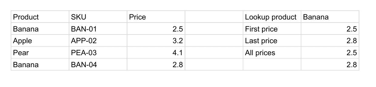
For example, if product names are in A2:A5, prices are in C2:C5, and the product you want is in F1, use =XLOOKUP(F1,A2:A5,C2:C5,"Not found"). You can paste that directly into Sheets.

How XLOOKUP works in Google Sheets

The basic formula has three arguments: what you want to find, where Sheets should look, and where it should take the answer from.

=XLOOKUP(search_key, lookup_range, result_range)

For the example below, F1 contains “Banana”. Sheets searches A2:A5 and returns the price from the same row in C2:C5. The two ranges need to line up: both must have the same number of rows, or the same number of columns if you search across a row.

=XLOOKUP(F1,A2:A5,C2:C5,"Not found")

That returns 2.5. There are two Banana rows, and the default search starts at the top. The optional fourth argument gives you a readable answer when there’s no match. Without it, Sheets returns #N/A. Exact matching is the default.

Find the last match instead

If newer entries sit below older ones, you may want the last match. Add 0 for exact matching and -1 for a search from the bottom up.

=XLOOKUP(F1,A2:A5,C2:C5,"Not found",0,-1)

In the example, that returns 2.8, the price on the second Banana row. Google Sheets also has approximate and wildcard match settings, but for ordinary names and IDs, I’d start with an exact match.

Return every match with FILTER

XLOOKUP finds one matching position. If you want every matching row, use FILTER instead.

=FILTER(C2:C5,A2:A5=F1)

That spills 2.5 and 2.8 into two cells. Leave the cells below the formula empty so the results have room. If nothing matches, FILTER returns #N/A; wrap it in IFERROR if you want a message instead.

XLOOKUP versus VLOOKUP, INDEX/MATCH, and QUERY

• XLOOKUP is the clearest choice for one result. The search column can sit to the left or right of the result column, and you don’t need to count column numbers.
• FILTER is better when several rows can match and you want all of them.
• VLOOKUP still works in existing sheets. You don’t need to replace a working formula just because a newer one exists, though its numbered result column can be awkward when a table changes.
• INDEX(MATCH) remains an option when you share a workbook with someone using older spreadsheet software.
• QUERY is better suited to selecting, grouping, or sorting a larger set of rows than to a single lookup.

The Google Sheets XLOOKUP reference lists the optional match and search settings. If you’re working with structured data, you can also make a native table in Google Sheets and refer to its columns by name.

The short answer

Use =XLOOKUP(value,where_to_search,where_to_return) for one matching answer. Add a fourth argument for a missing-value message. Add 0,-1 at the end when the last exact match is the one you need.