How to Make a Table in Google Sheets (Native Tables)

To make a table in Google Sheets, select your data and choose Format → Convert to table. Sheets gives you a named table with column controls, formatting, and views. You can also use the table name in formulas instead of keeping track of cell letters.

I use a table when I expect a list to grow or when I want formulas that are easy to read. For a quick calculation in an ordinary range, a table is optional.

Make a table from existing data

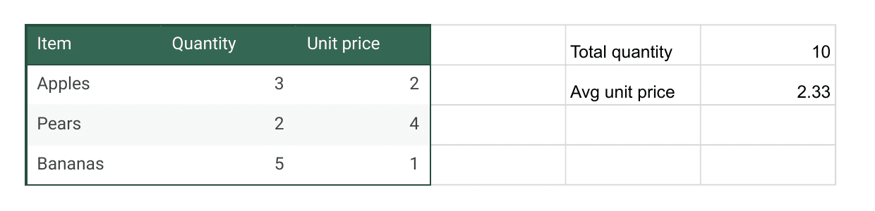
Put a clear heading at the top of each column. In my example, the headings are Item, Quantity, and Unit price. Then:

1. Select the cells you want in the table, including the headings.
2. Choose Format → Convert to table.
3. Check the range and the detected column types. Sheets adds a table name above the headings.
4. Click the table name and give it a name you’ll recognise later. I called mine Groceries.

I ran those steps in Sheets. The result is a real table, with a header for each column and controls for sorting and filtering. You can also start with a pre-built table from the Insert menu if a template suits your data.

Name the table and use its columns in formulas

A table reference names the table and the column in square brackets. To add the quantities in my example, I typed:

=SUM(Groceries[Quantity])

That returns 10. To get the average unit price, rounded to two decimal places, I used:

=ROUND(AVERAGE(Groceries[Unit price]),2)

That returns 2.33. These formulas keep pointing to the named column when you add or remove rows in the table. It’s much easier to read Groceries[Quantity] than to remember whether quantities are in column B or C. Google’s table reference guide has the full syntax.

If you need a value from another row, XLOOKUP works in Google Sheets. If you just want to add an ordinary column, see my SUM guide.

Set column types

Open the menu beside a column heading and choose Edit column type. You can mark a column as a number, date, dropdown, checkbox, or another supported type. Sheets then warns you when an entry doesn’t match that type. If a column genuinely mixes kinds of data, leave it as None.

Filter, sort, and group the table

Each column heading has a menu for sorting and filtering. For a separate way to examine the same data, open Views beside the table name and create a filter view. A group by view can collect rows by a chosen column and calculate totals or counts. Google’s table guide walks through those controls.

When a plain range is enough

If you only need to sort or filter a small, fixed range, Data → Create a filter is still fine. Converting it to a table makes more sense when you want named columns, column types, or views that you’ll keep using.

There are limits. Google says table references don’t yet work when you select ranges for charts, pivot tables, or conditional formatting. Use an ordinary cell range for those jobs. The table itself can still hold the source data.

The short answer

Select your headings and data, then choose Format → Convert to table. Name the table and use references such as Groceries[Quantity] in formulas. You get the table structure without building it out of named ranges and formatting tricks.